Advanced Functionalities
Using OSeMOSYS with the solver CPLEX
CPLEX is a commercial solver, more performing than the freely available GLPK solver for large problems. It is freely available for use by universities and in non-commercial projects. To run OSeMOSYS using CPLEX, you need to have CPLEX and Python installed on your PC.
- In order to use CPLEX, the OSeMOSYS model and data files first need to be combined into a single ‘.lp’ file. To do this, open the command prompt, select the GLPK folder containing the OSeMOSYS model and data files (see … for basic command prompt functions and how to select folders) and use the following command: glpsol -m [OSeMOSYS model file] -d [Data file] - -wlp [Input_Filename.lp]
- After the .lp file is generated, close the command prompt window. Open CPLEX. Type ‘read C:Input_FilepathInput_Filename.lp’ and press Enter. The command will require from few second, up to minutes to be executed, depending on the size of the file to be read from the chosen filepath.
- After the file is read, type ‘optimize’ and press enter. CPLEX will run the problem and find an optimal solution (or give a message of non-feasibility if no solution can be found).
- After the optimization is over, type ‘write C:Output_FilepathOutput_Filename.sol’ and press Enter. The command will require from few second, up to minutes to be executed, depending on the size of the file to be written to the chosen filepath. When the solution file is written, close the CPLEX window.
- The solution file needs now to be sorted and reordered. For this, download from the OSeMOSYS website the Python sorting script (bottom page) that was developed for this function and copy it in to the Python installation folder. Usually, when Python is installed, the folder ‘C:PythonXX’ is chosen by default. For this step and the next two, the instructions will assume this as the folder. Please check what the path of the installation folder is in your case and use that in steps 5, 6 and 7 instead, if different. Copy in the same folder also the Output_Filename.sol generated in the steps before.
- Open the command prompt again. Select the directory ‘C:PythonXX’ and type: python transform_31072013.py Output_Filename.sol Output_Filename.txt. The execution of the command may take from few seconds to minutes, depending on the size of the file.
- After the command is executed, type: ‘sort/+1<C:PythonXXOutput_FilepathOutput_Filename.txt>C:PythonXXOutput_Filename_so rted.txt’.
The file produced through the above process is available in the ‘C:PythonXX’ installation folder. The user may cut and paste it where she/he finds it convenient. It contains the results of the model run in a format that is easy to analyze, either directly or after copying into another platform such as MS Excel.
Modifications, enhancements and extensions of the main code
A number of extensions of the published version of the OSeMOSYS code were developed over time by different users from the community. They are briefly described in the following sub-sections. Information is provided on where to find the code, test case-studies (if available) and other relevant documentation.
Reduction of the translation time
One of the highest barriers to the creation of large continental models with detail to the country level, or highly detailed national applications, is the time and memory requirement to translate a model into a solvable matrix. In order to increase the applicability of the tool, a revision of the OSeMOSYS code was completed in late 2016, as the result of a public call launched and led by UNite Ideas.
Much of the flexibility of OSeMOSYS arises from the broad definition of all energy components as technologies and all energy carriers as fuels. The connections between them are specified in the data file by the user in the form of region- and time-specific tensors named Input- and OutputActivityRatio, that define the rate at which each fuel goes in and comes out of an active technology. Since in the majority of cases each technology converts one fuel into another – e.g. a gas turbine turning gas into electricity – the expected density of these tensors is very low, on the order of 1 over |regions| × |technologies| × |modes| × |fuels|. While previous versions of OSeMOSYS already filtered out technology-fuel relations with a zero rate and presented a straightforward linear problem to the solver, the amount of time used by having to apply this filter was repeatedly underestimated.
The updated version speeds this process up by generating intermediate parametric sets from a single scan over the sparse connection tensors after reading in the data file. These sets hold all the combinations of technology and modes of operation which consume or produce a specific fuel, and the rest of the model definition refers to them exclusively when considering technologies and fuels without any loss of generality. The updated version of OSeMOSYS including these changes is available on GitHub [1] .
All measures combined have been shown to reduce the time for translating the MathProg language of a reference country case-study from 526 seconds to 38 seconds on an Intel Core i5-2520M processor, a factor of 13; other cases show a similar speed-up. The subsequent time for solving the model is not affected. Further, when the code adjustments were tested on one of the largest OSeMOSYS models, the TEMBA model, considering the electricity supply system of 47 African countries, the sum of the translation and the calculation time was reduced from 18 hours to under 2 hours.
Short-term operational constraints of power plants
The global push towards increasing the share of Renewable Energy Sources (RES) in the energy supply poses challenges in terms of security and adequacy of electricity networks. Intermittent generation from e.g. wind and solar power may require back up. Two of the widely discussed options include controllable fossil fuel-fired generation (such as Open Cycle or Combined Cycle Gas Turbines) and storage. In order to assess the costs and benefits of using the first as a back-up option for peaking generation, new blocks of functionality computing short-term costs and operational constraints of dispatchable generation were designed. These include:
- Computing the reserve capacity dispatch to meet an exogenously given demand, under constraints on ramp rates and minimum duty [#welsch1]_ : the enhanced version of OSeMOSYS was compared to a modelling framework coupling TIMES and PLEXOS, through a case-study analysing optimal energy infrastructure investments in Ireland in 2020 [3] . While avoiding the high computational burden of the TIMES-PLEXOS model (the time resolution of the latter is 700 times higher), the OSeMOSYS model provides similar results. For instance, the investments diverge by 5%. The new block of functionality was further modified to make the reserve capacity demand an endogenous variable, namely a function of the penetration of intermittent renewables [4] .
- Costs related to the flexible operation of power plants, specifically: increased specific fuel consumption at lower load, wear and tear costs associated to the number of ramp-up and ramp-down cycles and costs for refurbishing existing units [5] .
Demand-flexibility
The expansions of the OSeMOSYS code introduced in Section 6.2.2. allow for the modelling of flexible supply options to back up the increasing intermittent renewable generation in energy systems. However, the transition to low-carbon and highly renewable energy systems can be facilitated also by demand-side options. Welsch et al. proposed an expansion to the code of OSeMOSYS, to allow for the modelling of elements of Smart Grids. The description of the enhancements is provided in [6] and the code formulation in the attachments to the same publication. The enhancements are compatible with the version of the OSeMOSYS code dated 8 November 2011 and available at www.osemosys.org. They include:
- Variability in generation. The CapacityFactor parameter is made timeslice-specific. This modification is embedded also in the currently published version of OSeMOSYS.
- Improved storage representation. Block of equations adding detail to the previous formulation for the storage. This modification is embedded also in the currently published of OSeMOSYS.
- Prioritizing demand types. Block of equations allowing the cost-optimal amount of load shedding and its overall cost to be computed, for certain flexible demand types defined by the user.
- Demand shifting. Block of equations allowing part of the demand to be shifted earlier or later in a day. The demand shift has a cost defined by the user and it can be constrained to occur within a certain time frame and up to a certain quantity.
Short-term planning
This version of OSeMOSYS was developed to further evaluate the short-term performance characteristics of systems with a high penetration of variable RES. It stems from the original code, enhanced by both the short-term operational constraints and the storage block of functionality described above. A number of additional modifications were introduced in order to improve the applicability of OSeMOSYS to finer time resolutions. Their focus was to preserve the temporal sequence of renewable energy availability and to evaluate the reaction of storage and other system management techniques to these dynamics. Specific changes include:
- Revised storage equations that are more computationally efficient for short-term modelling. Specifically, the intra-time slice storage equations in the base OSeMOSYS code were replaced with inter-time slice equations. This allows for much faster computation of the storage levels and allows for a larger number of scenarios to be computed in a shorter amount of time.
- Equations that model the ramping constraints of conventional generators. With large penetrations of variable renewables, the ramping demand in the system is significantly increased. The ability to constrain the ramping capabilities of generators in the system allows for a more accurate representation of the system dynamics and associated costs.
- Equations that incorporate the cost of curtailment into the model. This is not usually accounted for in a long-term model due to the averaging imposed by the time slice definitions.
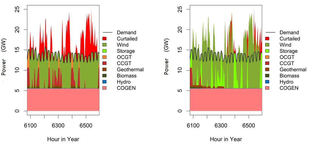
Comparison between the power generation profile without and with storage.
The Figure above shows results obtained when using OSeMOSYS for short-term planning. The curtailed energy is marked in red above the demand line. Energy stored for future use is shown in light green.
Stochastic modelling of energy security assessment
This extension was developed by Linas Martišauskas [7] . It aims to assess the amount of unsupplied energy and its costs, in case disturbances to the energy system occur. The extension consists of two parts:
- Stochastic model of disturbances. A probability distribution is created for several potential disturbances and scenarios are generated by randomly picking realisations of the disturbances. This module is external to OSeMOSYS and written in Matlab.
- Energy system optimization in the presence of disturbances. Block of equations to compute the system-wide unsupplied energy and its cost, for each of the disturbance scenarios generated through the stochastic model. This part constitutes an extension of OSeMOSYS and it can be directly embedded in the code.
The two modules are described in detail in the related Doctoral dissertation [7] .
Cascaded water storage
This addition to the basic OSeMOSYS storage equations allows for cascaded facilities to be included with an upper reservoir and generation station feeding water into a lower reservoir for a second generation station. Further, it is designed to track the storage levels and water flows, in and between each reservoir. Constraints representing minimum and maximum output flows from each dam are included to model both flood control and fish habitat management. Specific focus was put on maintaining a similar storage structure as the base OSeMOSYS code while providing a more user friendly formulation for modelling hydroelectric generation.
This application has proven important in the study of integrated approaches for the management of water and energy resources [8] .
The cascaded hydro storage equations have been uploaded to GitHub where anyone interested can download, use and modify them for their own purposes [9] .
| [1] | Optimus.community, OSeMOSYS GitHub, (2017). https://github.com/KTH-dESA/OSeMOSYS (accessed October 3, 2017). |
| [2] | Welsch, M., Howells, M., Hesamzadeh, M., O Gallachoir, B., Deane, P., Strachan, N., Bazilian, M., Kammen, D., Jones, L., Strbac, G., Rogner, H., 2015. Supporting security and adequacy in future energy systems: The need to enhance long-term energy system models to better treat issues related to variability. Int. J. Energy Res., 39, pp. 377–396. doi:10.1002/er.3250. |
| [3] | Welsch, M., Deane, P., Howells, M., O Gallachoir, B., Rogan, F., Bazilian, M., Rogner, H., 2014. Incorporating flexibility requirements into long-term energy system models–A case study on high levels of renewable electricity penetration in Ireland. Applied Energy, 135, pp. 600–615. doi:10.1016/j.apenergy.2014.08.072. |
| [4] | Maggi, C., 2016. Accounting for the long term impact of high renewable shares through energy system models: a novel formulation and case study. Politecnico di Milano [Online]. Available at: https://www.politesi.polimi.it/handle/10589/125684. |
| [5] | Gardumi, F., 2016. A multi-dimensional approach to the modelling of power plant flexibility. Politecnico di Milano. |
| [6] | Welsch, M., Howells, M., Bazilian, M., DeCarolis, J., Hermann, S., Rogner, H., 2012. Modelling elements of smart grids–enhancing the OSeMOSYS (open source energy modelling system) code. Energy, 46, pp. 337–350. doi:10.1016/j.energy.2012.08.017. |
| [7] | (1, 2) Martišauskas, L., 2014. Investigations of Energy Systems Disturbances Impact on Energy Security. Kaunas University of Technology and Lithuanian Energy Institute [Online]. Available at: http://www.lei.lt/_img/_up/File/atvir/2014/disertacijos/Santrauka_Martisauskas.pdf (accessed February 8, 2018). |
| [8] | de Strasser, L., Lipponen, A., Howells, M., Stec, S., Bréthaut, C., 2016. A Methodology to Assess theWater Energy Food Ecosystems Nexus in Transboundary River Basins. Water, 8, 59. doi:10.3390/w8020059. |
| [9] | Niet, T., 2017. GitHub - tniet/OSeMOSYS. Available at: https://github.com/tniet/OSeMOSYS (accessed October 7, 2017). |